Matplotlib 学习笔记
安装
随便找了一个教程,这部分很简单,没有大问题
基本用法
1 | import matplotlib.pyplot as plt |
figure 图像
- plt.figure(num=3,figsize=(8,5)) num表示序号,是第几个图,figsize表示大小,长和宽
- plt.plot(x,y1,color=’red’,linewidth=5.0,linestyle=’–’) color表示线的颜色,linewidth表示线的宽度,linestyle表示类型,虚线用–表示
设置坐标轴
- plt.xlim((-1,2)) plt.ylim((-1,3)) 设置x或y轴的取值范围
- plt.xlabel(‘x’) plt.ylabel(‘y’) 设置坐标轴表示
- new_ticks=np.linspace(-1,2,5)
- plt.xticks(new_ticks) 设置坐标轴的值
- plt.yticks([-2,-1.8,-0.5,1,2],[r’$a\ \alpha c$’,r’$b$’,r’$c$’,r’$d$’,r’$e$’])设置坐标轴的值和标识
- ax = plt.gca() 图像的边框
legend 图例
1 | l1, = plt.plot(x,y2,label='up') |
handles表示需要legend的线条,labels表示legend中线条的名称,loc表示位置,best可以自动选区最好的位置。
annotat 注解
1 | import numpy as np |
tick 能见度
1 | for label in ax.get_xticklabels() + ax.get_yticklabels(): |
注意dict中的参数zorder表示是哪一个图层
scatter 散点图
1 | import matplotlib.pyplot as plt |
X,Y是由numpy产生的随机数组,c为颜色模式,alpha为能见度
Bar 柱状图
1 | import matplotlib.pyplot as plt |
Contours 等高线图
1 | import matplotlib.pyplot as plt |
image图片
1 | import matplotlib.pyplot as plt |
3D plot
1 | import numpy as np |
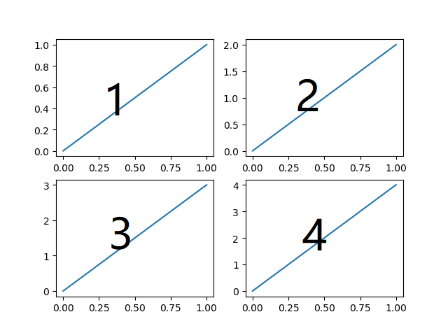
subplot多个显示
1 | # plt.subplot(行,列,位置序号) |
1
2
3
4
5
6
7
8
9
10
11
12
13
14
15
16
17import matplotlib.pyplot as plt
plt.figure()
plt.subplot(2,1,1)
plt.plot([0,1],[0,1])
plt.subplot(2,3,4)
plt.plot([0,1],[0,2])
plt.subplot(2,3,5)
plt.plot([0,1],[0,3])
plt.subplot(2,3,6)
plt.plot([0,1],[0,4])
plt.show()
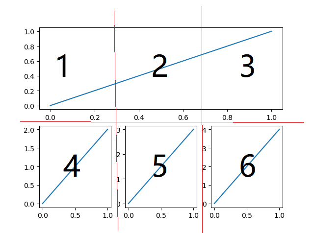
subplot 分格显示
method 1:subplot2grid
1 | import matplotlib.pyplot as plt |
plt.subplot2grid((3,3)表示形状,(2,1)图像左上角的位置,colspan=3 所占列,rowspan=1所占行)
method 2:gridspec
1 | import matplotlib.pyplot as plt |
method 3:easy to define structure
1 | import matplotlib.pyplot as plt |
传出的f可以用来调整窗口的格式,share表示是否共享坐标轴,
图中图
1 | import matplotlib.pyplot as plt |
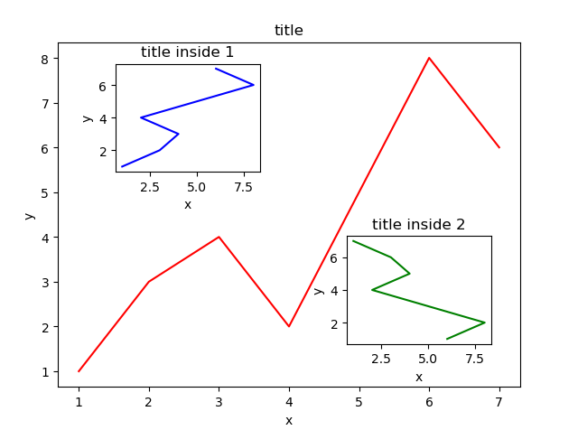
其实就是用行列位置+宽高尺寸所确定的绝对位置来布置图片,这里的尺寸是图片占窗口的百分比
次坐标轴
1 | import matplotlib.pyplot as plt |
animation 动画
1 | import numpy as np |
许多方法参数还需要在未来实践中慢慢摸索,matplotlib是真滴强大!!!Orz Orz Orz Orz Orz